Counting Incidents: Time Series and Category Counts • VietnamWarData

This article covers the other workhorse task with the combined data: counting incidents — over time (annual and monthly time series) and by category. As elsewhere, the code is shown but not executed at build time; the figures are pre-rendered.

Setup

library(VietnamWarData)
library(dplyr)
library(lubridate)
library(ggplot2)
library(scales)

incidents <- get_comb_inc_dta()

Incidents per year

Count by initiation_date year and aggressor_side. The 1968 Tet Offensive stands out as the peak of enemy-initiated activity.

incidents |>
  filter(!is.na(aggressor_side), between(year(initiation_date), 1963, 1973)) |>
  mutate(year = year(initiation_date)) |>
  count(year, aggressor_side) |>
  ggplot(aes(year, n, color = aggressor_side)) +
  geom_line(linewidth = 1) +
  geom_point(size = 2) +
  scale_x_continuous(breaks = 1963:1973) +
  scale_y_continuous(labels = comma) +
  scale_color_brewer(palette = "Set1") +
  labs(x = "Year", y = "Number of incidents", color = NULL)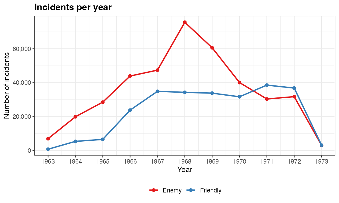

Incidents per month

lubridate::floor_date() collapses dates to the first of each month for a finer time series, faceted by side.

incidents |>
  filter(!is.na(aggressor_side), between(year(initiation_date), 1963, 1973)) |>
  mutate(ym = floor_date(initiation_date, "month")) |>
  count(ym, aggressor_side) |>
  ggplot(aes(ym, n)) +
  geom_col(fill = "grey35") +
  facet_wrap(~ aggressor_side, ncol = 1, scales = "free_x") +
  scale_x_date(date_breaks = "1 year", date_labels = "%Y") +
  scale_y_continuous(labels = comma) +
  labs(x = "Year", y = "Incidents / month")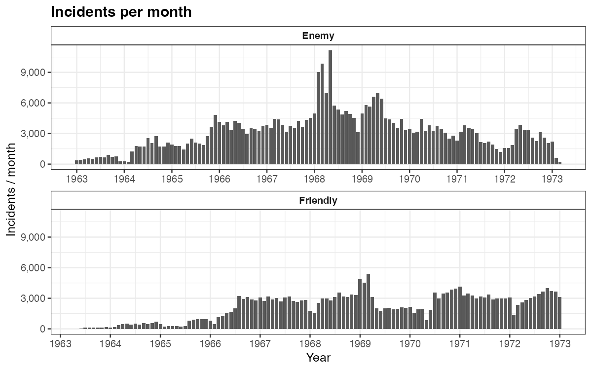

Incident counts by category

A simple count() ranks enemy-initiated incidents by enemy_action_category. reorder() sorts the bars; coord_flip() makes the labels readable.

incidents |>
  filter(aggressor_side == "Enemy", between(year(initiation_date), 1963, 1973)) |>
  mutate(
    enemy_action_category = coalesce(enemy_action_category, "Not categorized"),
    # tidy up a spelling artifact carried over from the source file
    enemy_action_category = recode(enemy_action_category, "Sabotoge" = "Sabotage")
  ) |>
  count(enemy_action_category) |>
  mutate(enemy_action_category = reorder(enemy_action_category, n)) |>
  ggplot(aes(enemy_action_category, n)) +
  geom_col(fill = "grey35", color = "black") +
  coord_flip() +
  scale_y_continuous(labels = comma) +
  labs(x = NULL, y = "Number of incidents")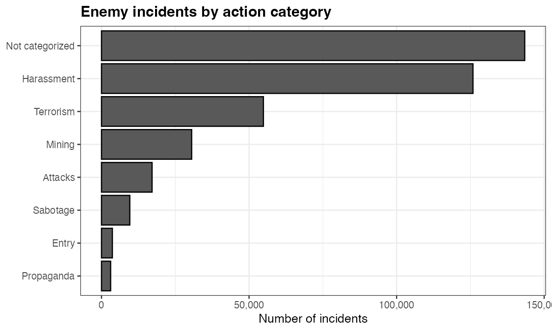

Where to go next

Swap aggressor_side for data_file_origin to see how each source file contributes over time.
Count a different column (e.g. general_action_category, prov_name) the same way.
Map these counts spatially with the province choropleth or satellite articles.